The universe as the addressing of a single e

The model proposes an alternative structural reading of the universe — not a correction of the Standard Model, but a reading that stands on its own, built from a few fundamental pieces: a single e at t=0, a circular and constant axis T, a generative function 4df(x), and the outbound–return duality of energy-links.

Author: Gabriel Cantin Lanoraie, Quebec Phase 1 complete — Mathematical Phase 2 to be undertaken CC BY-NC-ND 4.0

Section 1 — Foundation

Founding overview

The model in one sentence: the entire universe is the addressing of a single e (at t=0) within an observation membrane t=x via a generative function 4df(x), inscribed on a circular and constant axis T. Everything we observe — particles, forces, masses, charges, dark energy, expansion — is a structural manifestation of this single mechanism.

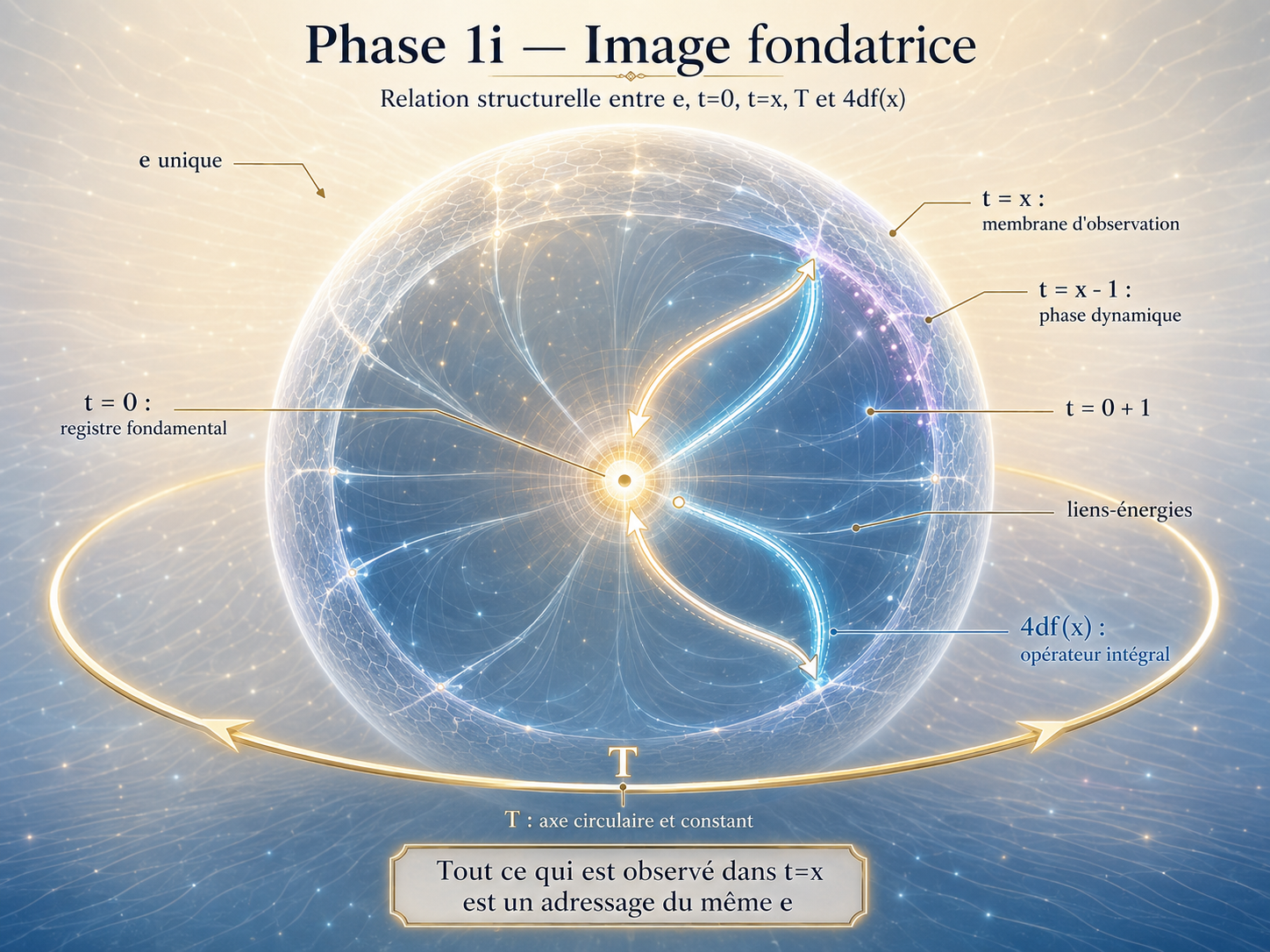
Founding image: structural relation between e, t=0, t=x, T and 4df(x) — Fig. 0 **Founding image — structural relation between e, t=0, t=x, T and 4df(x)** The single e at t=0 (fundamental register, outside sequence). T is circular and constant. 4df(x) is the integral operator that addresses e within the observation membrane t=x. Everything we observe in t=x is an addressing of the same e.

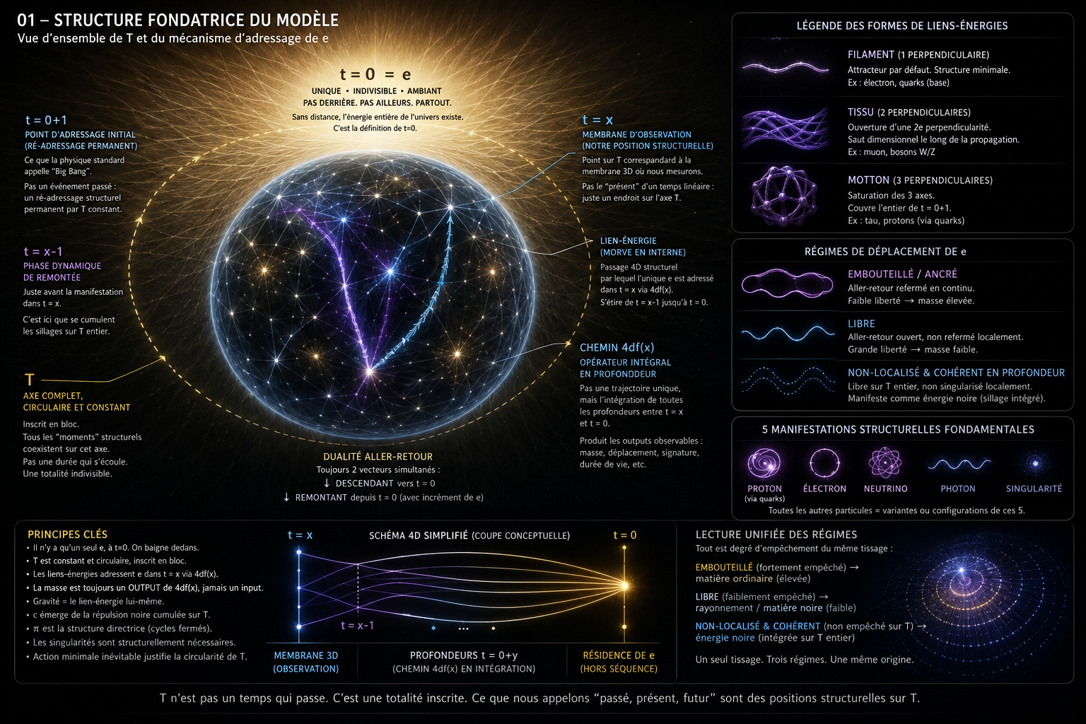
Founding structure: circular T, energy-link forms, manifestations — Fig. 1 **Founding structure of the model — overview of T and the addressing mechanism of e** Three forms of energy-links (filament 1D, fabric 2D, lump 3D), three displacement regimes (bottled, free, non-localized), five fundamental structural manifestations (proton, electron, neutrino, photon, singularity). Everything is a variation of a single mechanism.

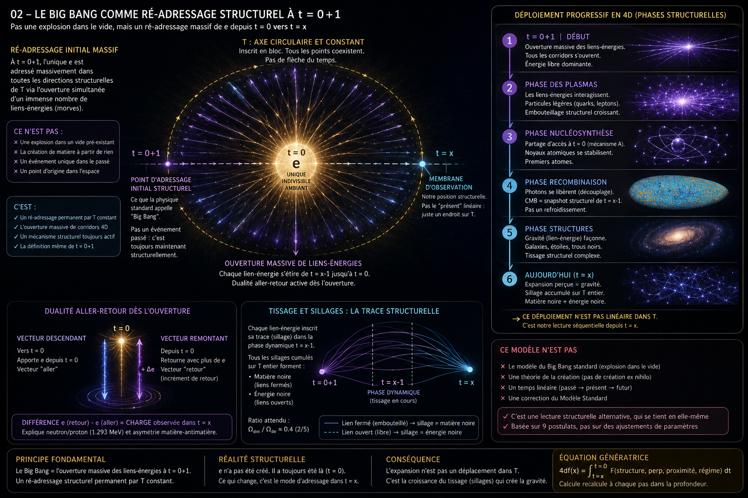
Fig. 2 **The Big Bang as structural re-addressing at t=0+1** Not an explosion in the void. A massive structural re-addressing of e from t=0 toward t=0+1. Progressive deployment in four dimensions: beginning, plasmas, nucleosynthesis, recombination. The deployment is not linear in T.

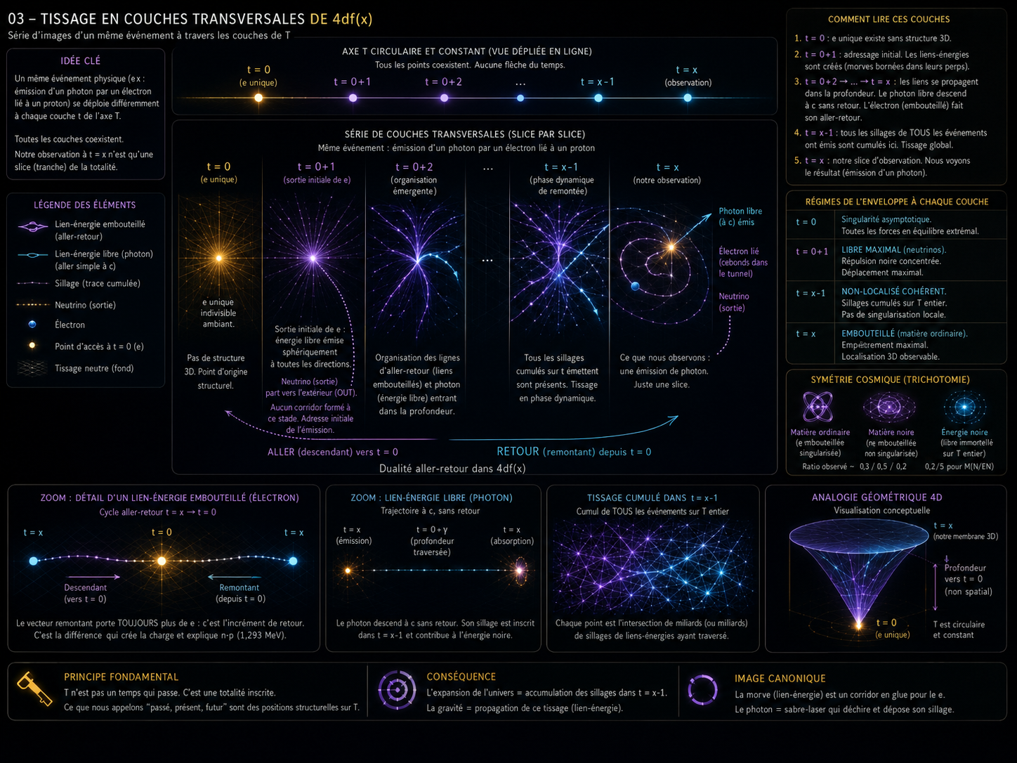
Fig. 3 **Weaving in transverse layers of 4df(x)** Unfolded view of T: all points coexist. The transverse layers show the outbound–return of every energy-link across depth. The 3D we perceive at t=x is a local reading of a weaving cumulated over the entirety of T.

Section 2 — Reading

Central structural warnings

These four warnings must be read before the genesis images. They correct the natural slippage toward a sequential, linear reading of the model.

1 · T is not a sequence — total duration determines the beginning T is a constant structural totality, not a flow. The first instants of the universe are not only "before": they are determined by the whole of T. The last hundreds of billions of years play a decisive role for e, because they correspond to an inverted duration of return, resolution, singularization, and re-addressing.

2 · Observation at t=x — reading at c — structural proximity to t=0 When we observe space, we don't directly see t=0+1. We observe proportions of t=x made visible by distance and information transported at c. A vector spanning ten billion years at t=x can remain relatively close to t=0 at the structural scale of T.

3 · No photons at the beginning — the universe at t=0+1 has no complete photons A photon is an open structure defined by its full existence over c. Three conditions for manifestation: (1) extension over c, (2) information transport at c, (3) reception possible at t=x. At t=0+1: none of the three is met. This is what makes e observable in t=x.

4 · At t=0+1: a single OUT — quarks are what is at play The photon's weaving is inscribed in whole T and arrives at t=x-1 ahead of t — but we never see it directly. At t=0+1, e is addressed in the quark mode (strong dimension, maximum proximity) and the neutrino mode (assembly in progress, observable at t=0+2). Not in the photon mode.

Section 3 — Structural genesis

From t=0 to t=x (A1 — A7)

The following images show the structural deployment from t=0 to the observation membrane t=x. Reading caution: these are not successive moments after the big bang. They are structural positions in whole T. Structural progression stops at t=0+3; beyond that, we are inside the membrane t=x where we read cumulative manifestations.

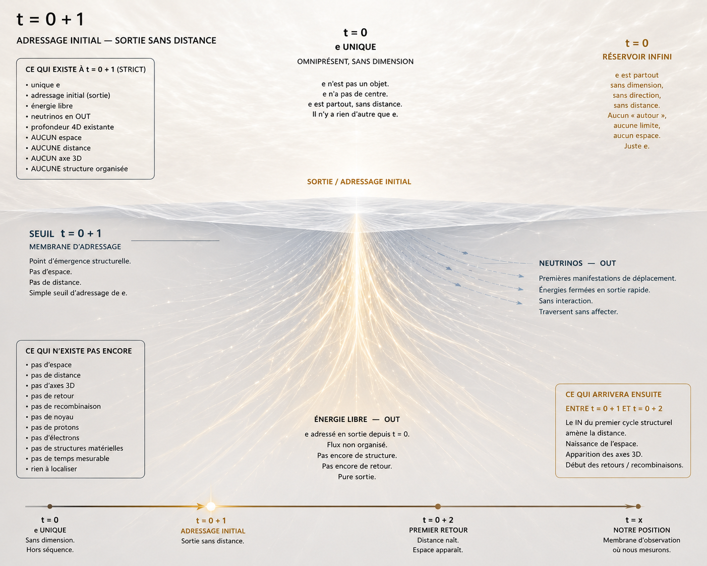
t=0+1: initial addressing, output without distance — A1 · t=0+1 **Initial addressing — output without distance** Free energy OUT, neutrinos OUT. No space, no distance, no 3D axes, no organized structure. Only the initial addressing of e at t=0+1. Addressing membrane: emergence threshold.

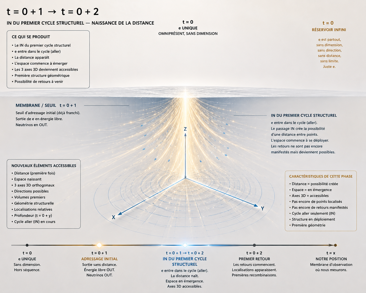
t=0+1 → t=0+2: birth of distance, immersive view — A2 · t=0+1 → t=0+2 **IN of the first structural cycle — birth of distance (immersive view)** Distance appears, space begins to emerge, the three 3D axes become accessible. First geometric structure. Atmospheric view of the structural shift.

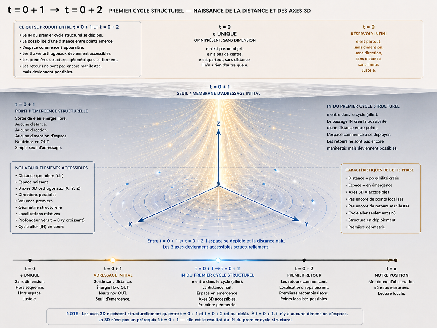
t=0+1 → t=0+2: birth of distance and 3D axes, didactic view — A3 · t=0+1 → t=0+2 **First structural cycle — birth of distance and 3D axes (didactic view)** Same events as A2 but with global timeline, explanatory boxes, and legends. Complete pedagogical angle on the shift.

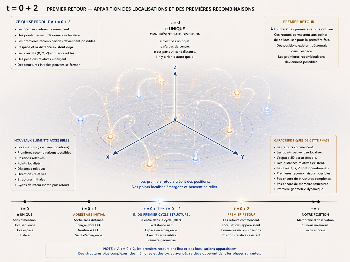
t=0+2: appearance of localizations and first recombinations — A4 · t=0+2 **First return — appearance of localizations and first recombinations** The X/Y/Z axes become accessible. Points can localize. First recombinations become possible. The neutrino becomes observable at t=0+2.

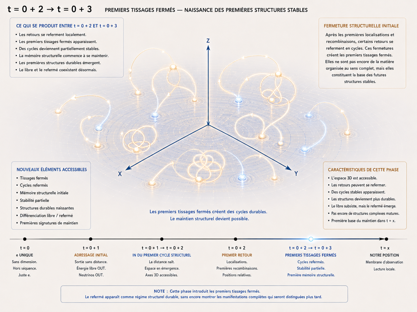
t=0+2 → t=0+3: first closed weavings, birth of stable structures — A5 · t=0+2 → t=0+3 **First closed weavings — birth of the first stable structures** Returns reclose locally. Partially stable cycles. Initial structural memory. Free and reclosed now coexist. First durable structures.

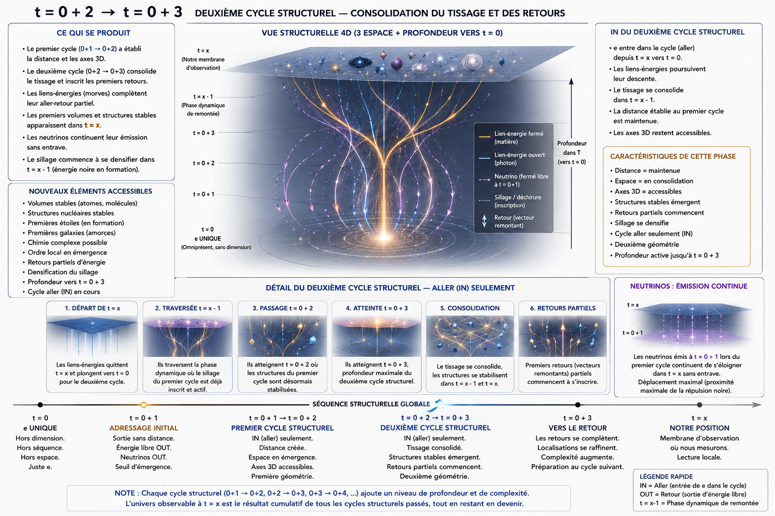
t=0+2 → t=0+3: second structural cycle, consolidation of weaving and returns — A6 · t=0+2 → t=0+3 **Second structural cycle — consolidation of weaving and returns** Consolidated 4D view. First volumes/stable structures appear in t=x. Continuous neutrino emission. The wake begins to densify in t=x-1 — dark energy in formation.

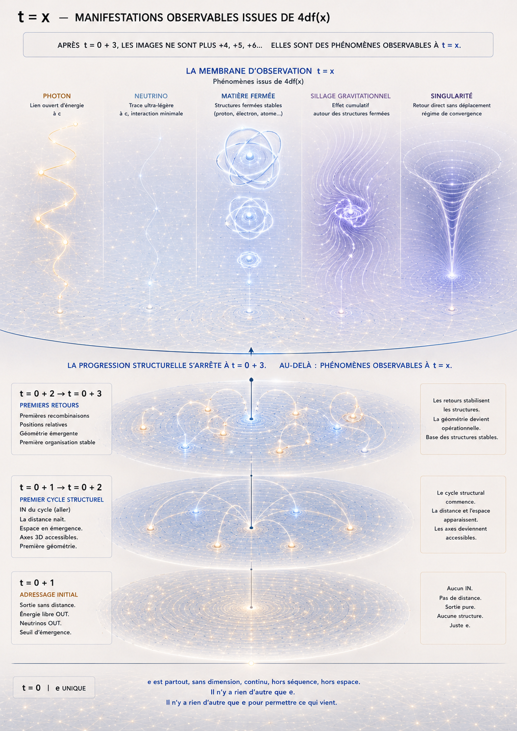
t=x: observable manifestations issued from 4df(x) — A7 · t=x — key image **Observable manifestations issued from 4df(x)** The five fundamental manifestations at t=x: photon (open energy-link at c), neutrino (ultra-light traces), closed matter (proton, electron, atoms), gravitational wake (cumulative effect around closed structures), singularity (direct return without displacement). *Structural progression stops at t=0+3. Beyond: observable phenomena at t=x.*

Section 4 — Particles and forces

B1 — B5: entanglement, forces, quarks, photon

This section applies the model to fundamental phenomena: entanglement (a sharing of anchoring at t=0, not a signal), the four forces re-read as weaving regimes, exotic quark chemistry at the LHC, the proton's stability, and the complete cycle of a photon emission.

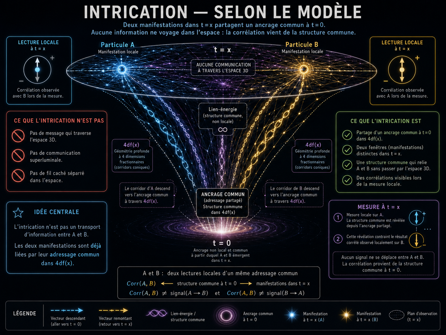
Entanglement according to the model: common anchoring at t=0 — B1 · Entanglement **EPR entanglement — sharing of anchoring at t=0** Two manifestations in t=x share a common anchoring at t=0. No information travels through space: the correlation comes from the shared structure in 4df(x). No superluminal communication — there is no separate e reaching the other.

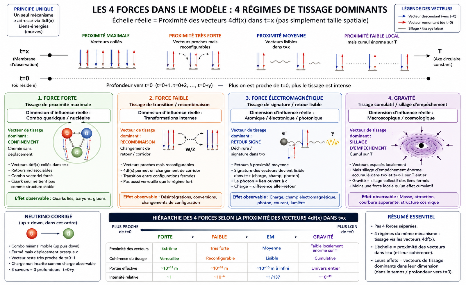
The 4 forces in the model: 4 dominant weaving regimes — B2 · 4 forces **The 4 forces in the model — 4 dominant weaving regimes** Not four separate forces — a single mechanism with four regimes according to the proximity of the 4df(x) vectors in t=x. **Strong** (maximum proximity, confinement); **weak** (very strong proximity, recombination); **electromagnetic** (medium proximity, signed return); **gravity** (locally weak proximity but enormous cumulative wake over whole T).

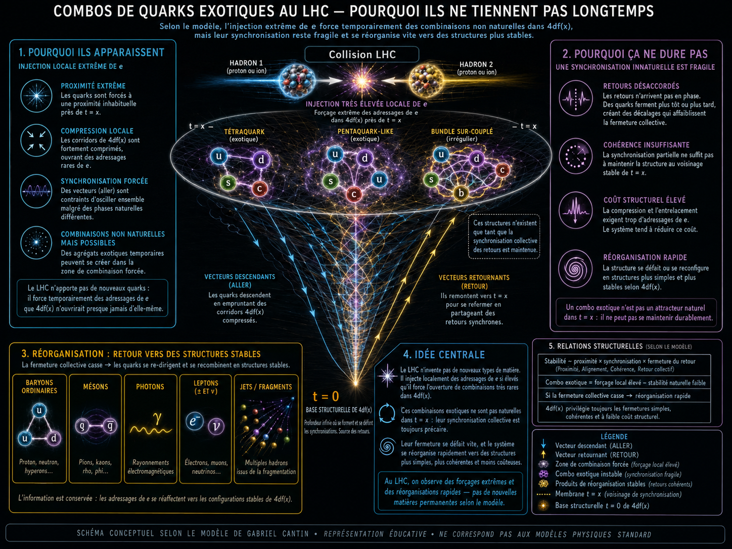
Exotic quark combos at the LHC: why they don't last — B3 · LHC **Exotic quark combos at the LHC — why they do not hold for long** The extreme injection of e temporarily forces non-natural combinations in 4df(x). Tetraquarks, pentaquarks, bundles: their synchronization remains fragile and quickly reorganizes toward stable structures (baryons, mesons, photons, leptons, jets). The LHC opens a window — it does not create.

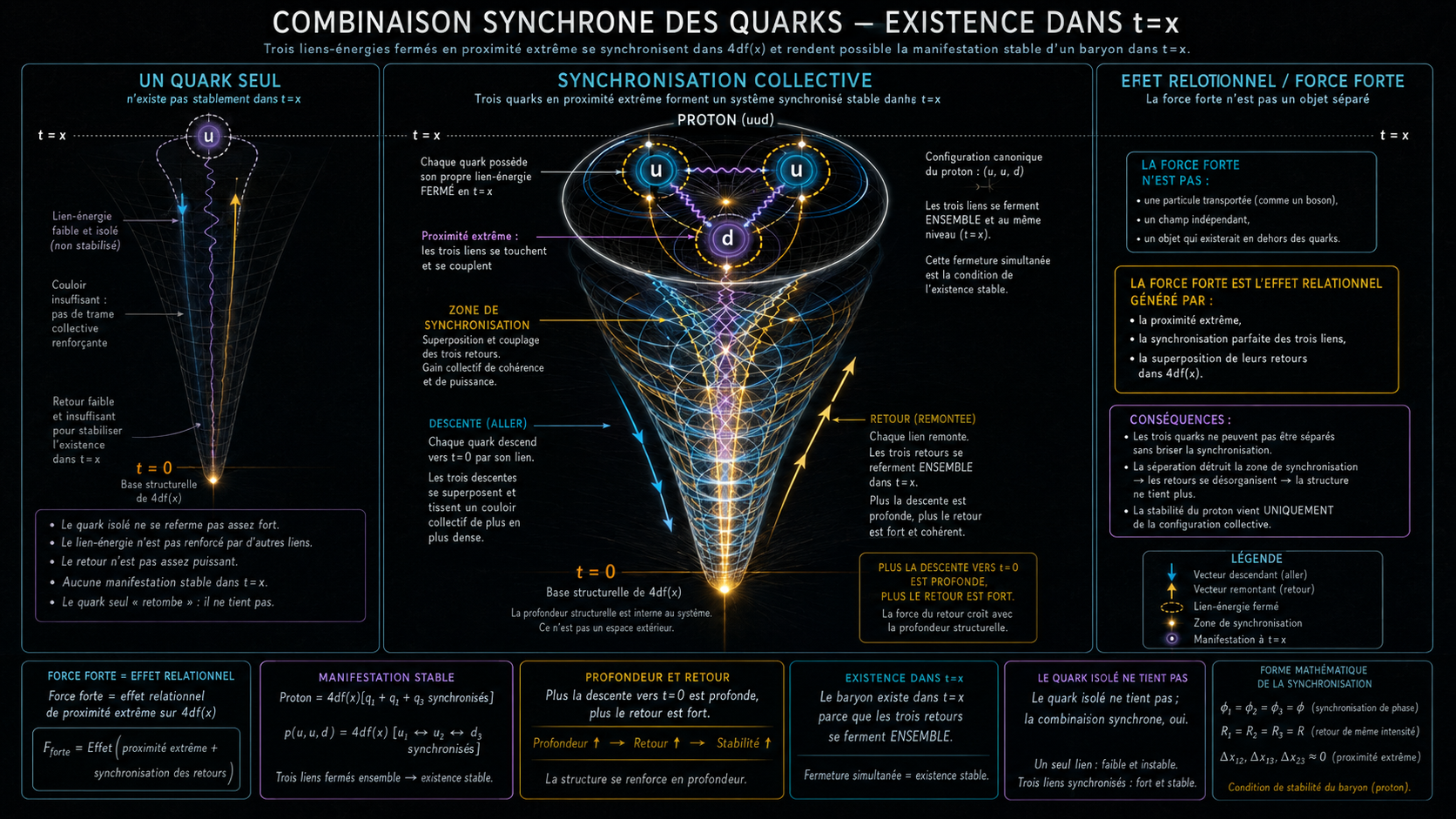
Synchronous combination of quarks: proton uud — B4 · Strong force **Synchronous combination of quarks — why the proton (uud) holds** A lone quark does not exist stably in t=x. Three quarks in extreme proximity form a stable synchronized system. The strong force is not a transported particle — it is the relational effect generated by extreme proximity, the synchronization of the three links, and the superposition of their returns in 4df(x).

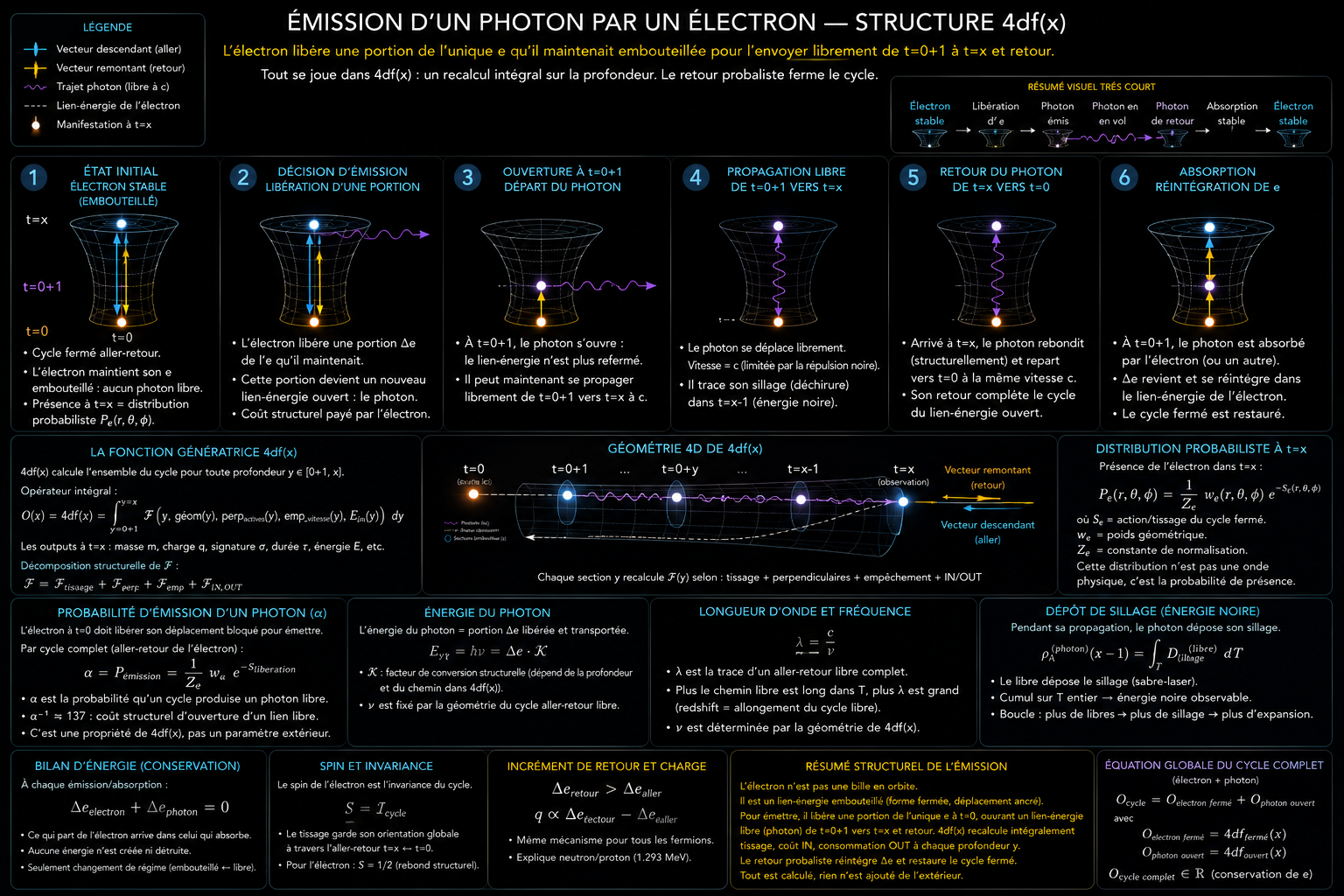
Emission of a photon by an electron: 4df(x) structure — B5 · Photon **Emission of a photon by an electron — 4df(x) structure** Six steps of the complete cycle: stable initial electron state, liberation of a portion, opening at t=0+1, free propagation, return, absorption. With conceptual equation proposals (energy, wavelength, wake deposit). The equations are illustrative — not Gabriel-derivations.

Section 5 — Structural readings

C1 — C7: charge, electron, reactions, angular force, first instants, T, 4df(x)

This section deepens the structural readings: what charge is, how the electron actually inhabits the nucleus, how to re-read standard reactions, what angular force is, why no photon yet at t=0+1, and how whole T and 4df(x) are to be read.

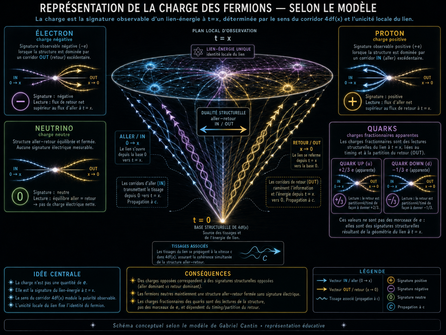
Representation of fermion charge according to the model — C1 · Charge **Representation of fermion charge** Charge is the observable signature of an energy-link at t=x, determined by the direction of the 4df(x) corridor and by the local uniqueness of the link. Electron (negative, OUT excess), proton (positive, IN excess), neutrino (neutral, outbound = return), quarks (apparent fractional charges = structural readings).

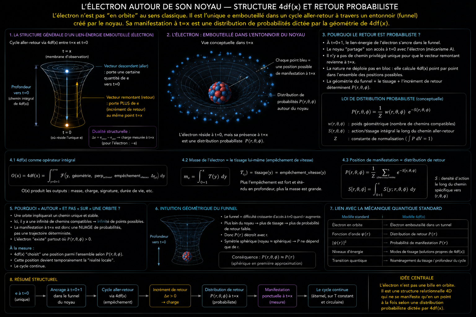
The electron around its nucleus: 4df(x) structure and probabilistic return — C2 · Electron **The electron around its nucleus — 4df(x) structure and probabilistic return** The electron is not in orbit: it is bottled in an outbound–return cycle through a funnel created by the nucleus. The return is probabilistic — it is the coupling that dictates it. Correspondence with standard quantum mechanics (orbit → tunnel, ψ(r) → return distribution, |ψ|² → manifestation probability).

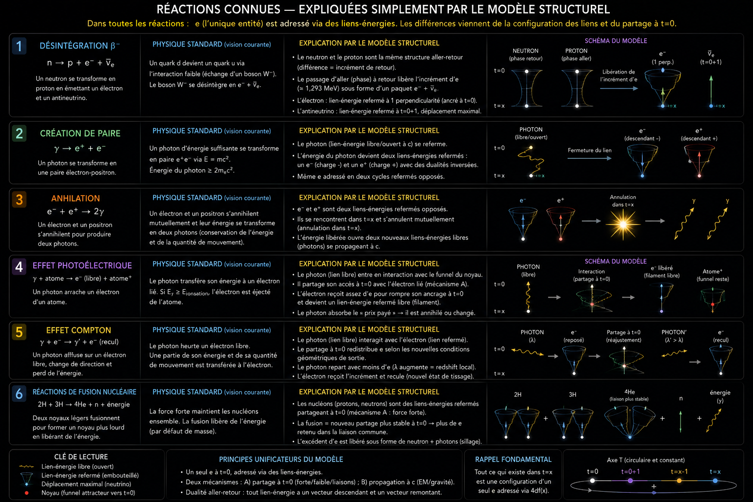
Known reactions explained by the structural model — C3 · Reactions **Known reactions — explained simply by the structural model** Six standard reactions re-read: β⁻ decay, pair creation, annihilation, photoelectric effect, Compton effect, nuclear fusion. Standard view vs. structural explanation. Everything comes from the configuration of energy-links and sharing at t=0.

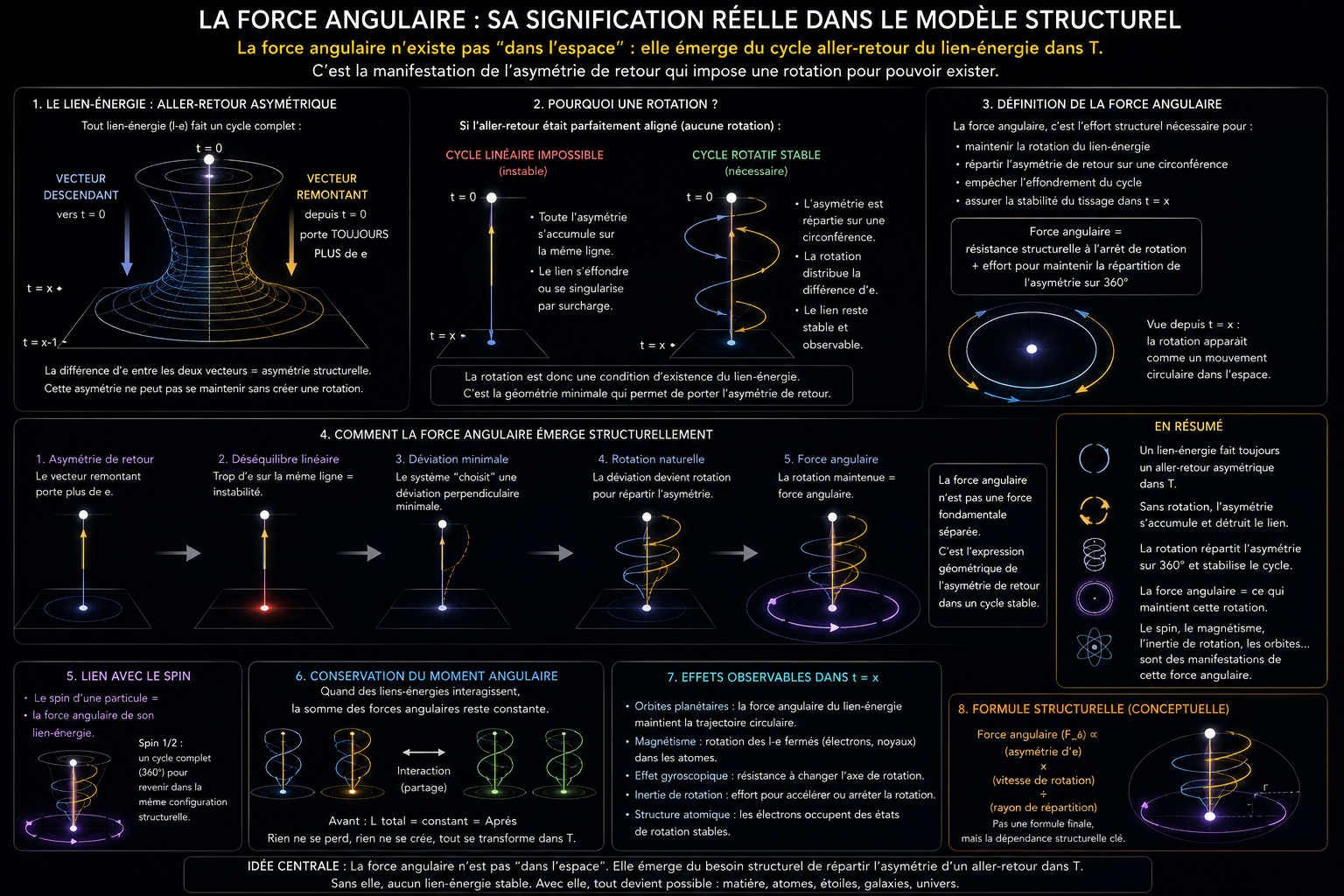
Angular force: its real meaning in the structural model — C4 · Angular force **Angular force — its real meaning** Angular force does not exist "in space." It emerges from the outbound–return cycle of the energy-link in T. It is the manifestation of return asymmetry that imposes rotation in order to exist. Without rotation, asymmetry accumulates and the link collapses/singularizes. With rotation, asymmetry distributes over 360°.

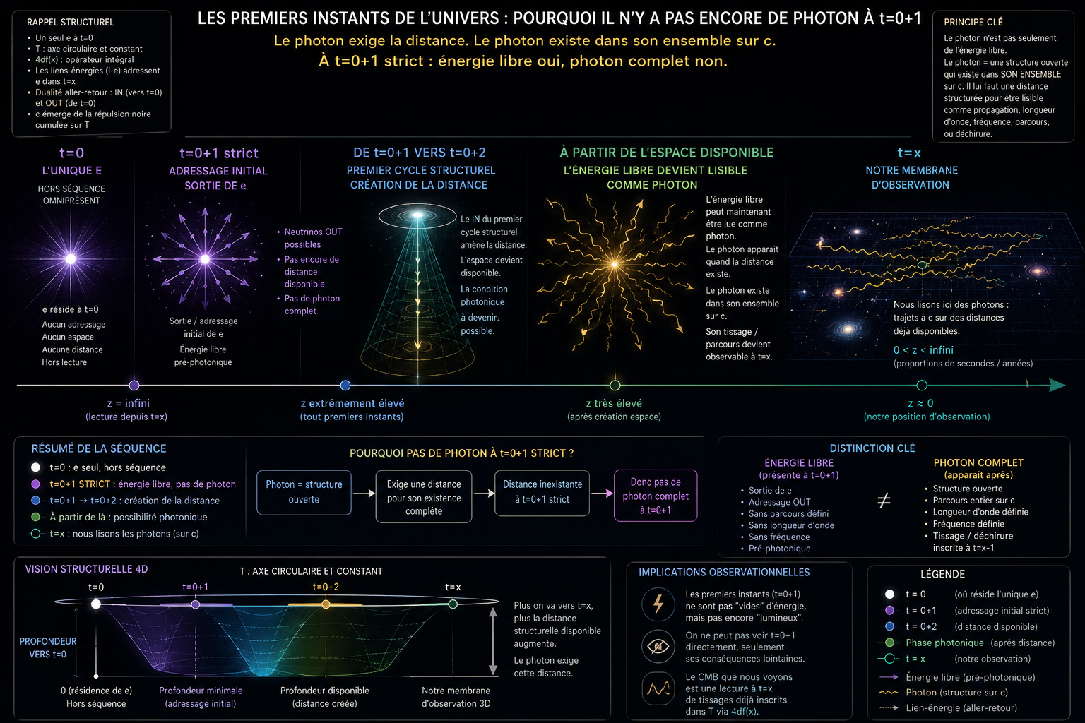
First instants of the universe: why there is no photon yet at t=0+1 — C5 · First instants **The first instants of the universe — why there is no photon yet at t=0+1** Distinction "free energy" vs. "complete photon." No distance available yet, no complete photon at strict t=0+1. Observational implication: the first instants are not empty of energy, but not yet luminous. The CMB is a reading at t=x of weavings already inscribed in T.

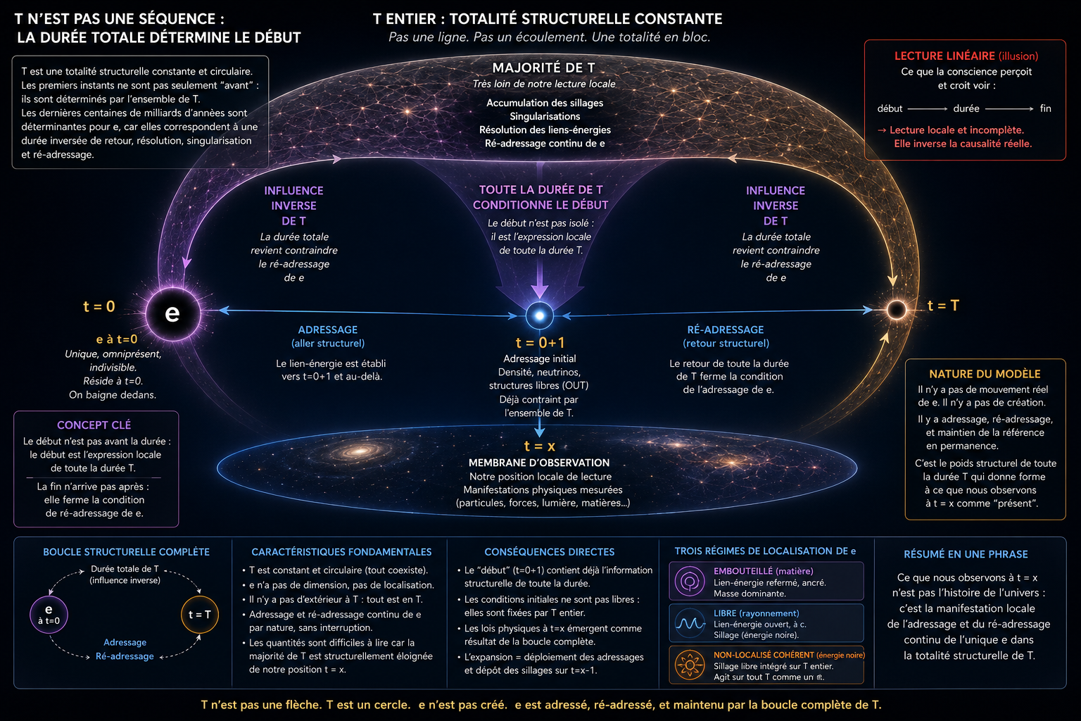
Whole T: constant structural totality — C6 · Warning 1 **Whole T — constant structural totality** T is not a sequence. Not a line, not a flow, a totality in block. Total duration conditions the beginning; inverse influence of T on the addressing of e. The beginning is not isolated: it is the local expression of the entire duration T.

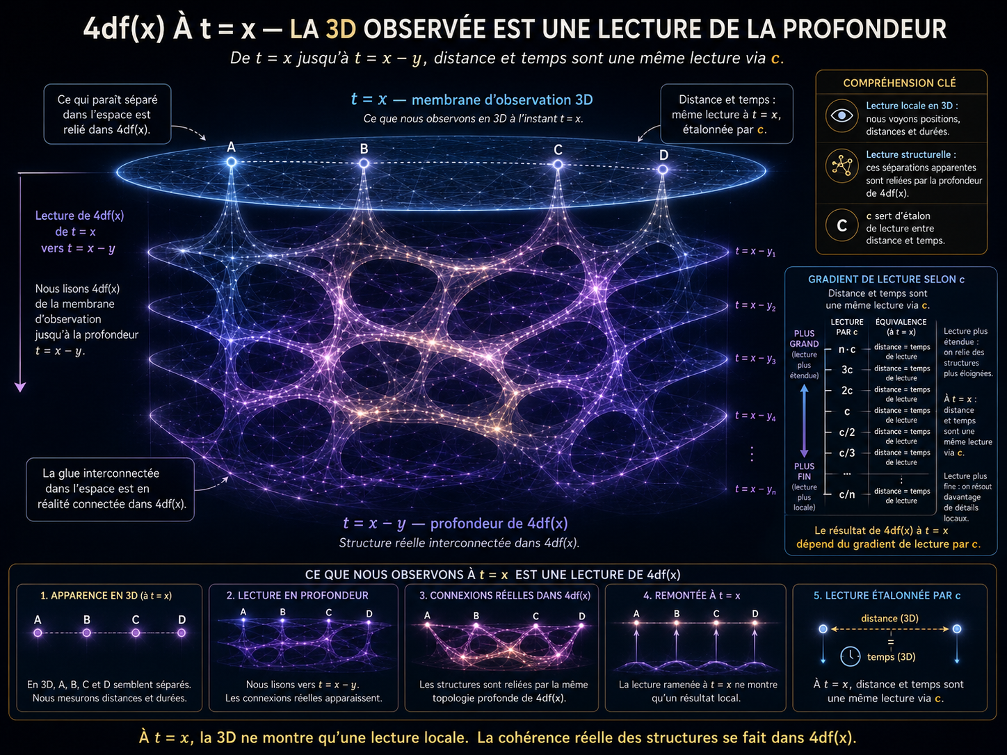
4df(x) at t=x: observed 3D is a reading of depth — C7 · 4df(x) **4df(x) at t=x — observed 3D is a reading of depth** From t=x down to t=x-y, distance and time are the same reading via c. 3D shows only a local reading; the real coherence of structures happens inside 4df(x). The deeper the descent, the stronger the return.

Section 6 — Additional pedagogy

D1 — D5: duality, sequential plan, reading at c, tennis-ball analogies

These images bring complementary angles useful for building intuition: the outbound–return duality seen as a funnel, the complete sequential plan of the model, the structural reading of T, and two "tennis-ball analogy" versions of the electron's cycle.

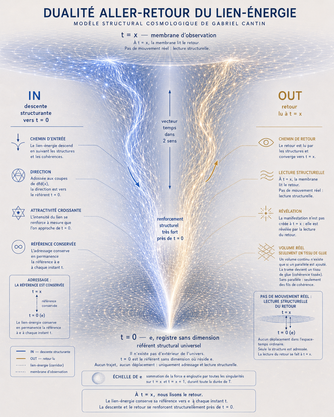
Outbound-return duality of the energy-link — D1 **Outbound–return duality of the energy-link** The energy-link has two simultaneously observable vectors at any t=x point: a descending one (IN, toward t=0) and a rising one (OUT, toward t=x). Intensity strengthens toward t=0. At t=x, we read the return. Charge = e-difference between the two vectors.

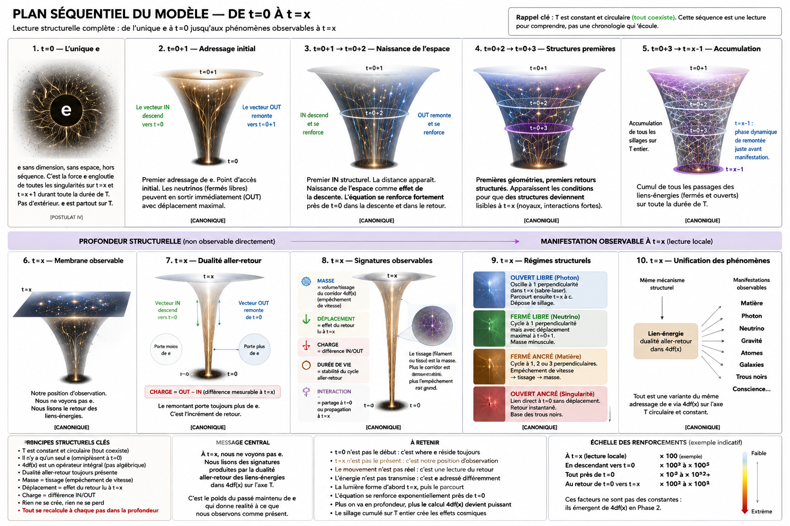
Sequential plan of the model from t=0 to t=x — D2 **Sequential plan of the model — from t=0 to t=x** Complete structural reading from the single e at t=0 down to observable phenomena at t=x. Structural depth not directly observable, then observable manifestation at t=x. The sequence is a reading, not a chronology.

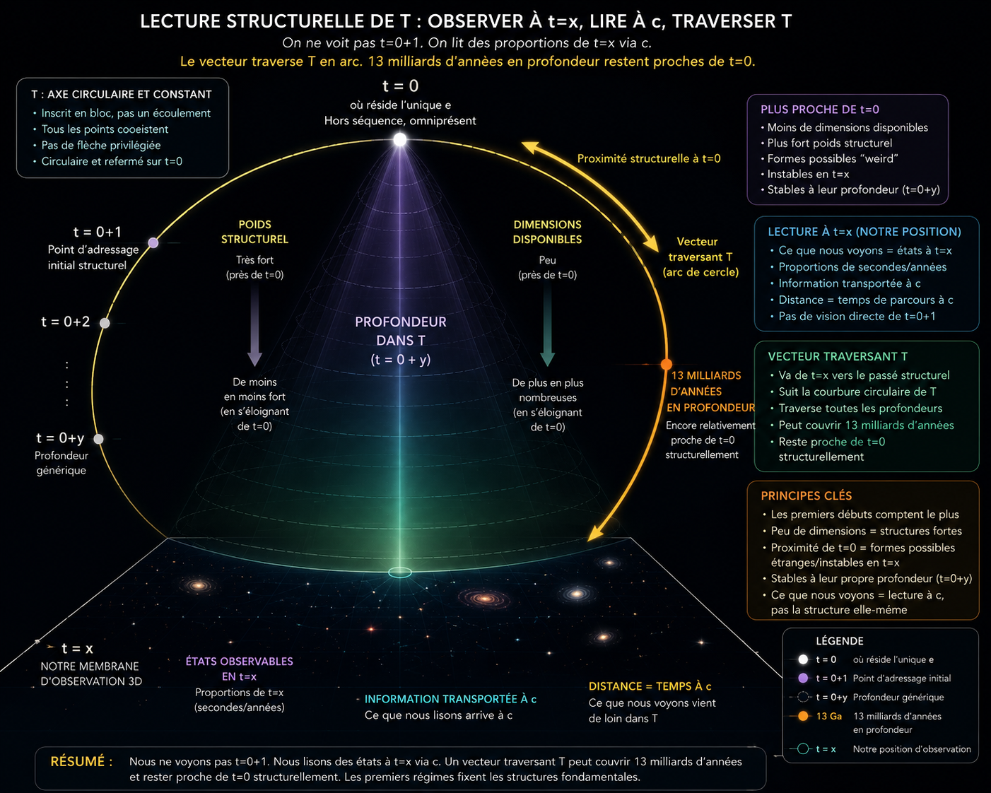
Structural reading of T: observe at t=x, read at c, traverse T — D3 · Warning 2 **Structural reading of T — observe at t=x, read at c, traverse T** We do not see t=0+1. We read proportions of t=x via c. A vector traversing T as an arc — for example 13 billion years in depth — can stay structurally close to t=0. The early regimes near t=0 strongly fix the fundamental structures.

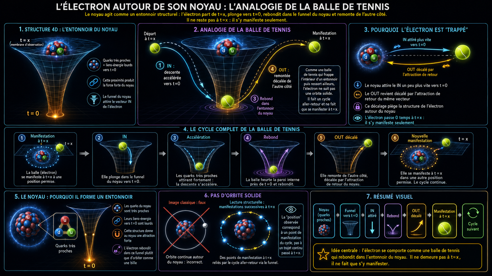
The electron around its nucleus: tennis-ball analogy — D4 · Analogy **The electron around its nucleus — tennis-ball analogy** The nucleus acts as a structural funnel. The electron leaves t=x, plunges toward t=0, rebounds in the nucleus funnel, and rises back on the other side. It does not stay at t=x: it only manifests there. Explicit rejection of the classical solid-orbit image.

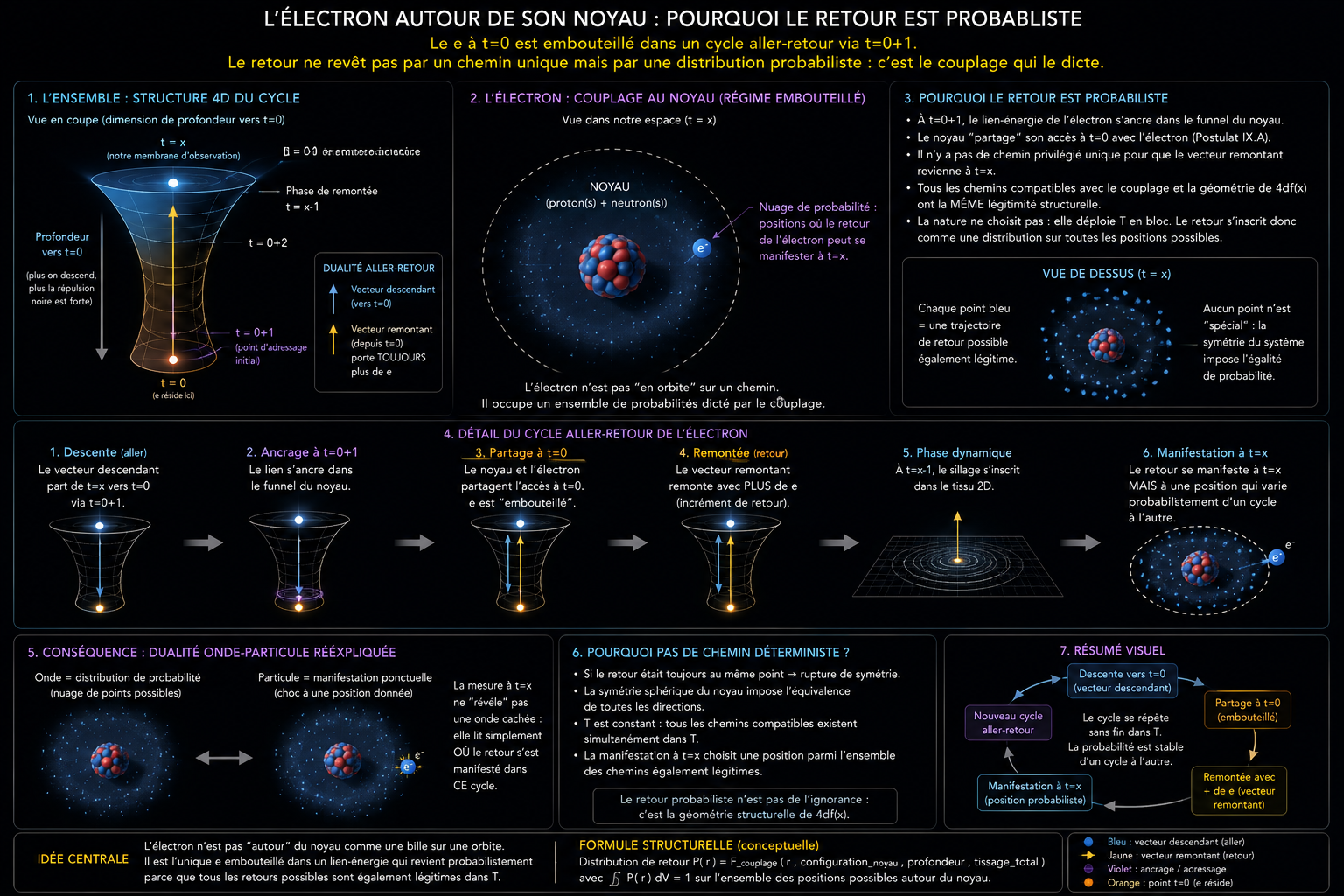
The electron around its nucleus: why the return is probabilistic — D5 · Probability **The electron around its nucleus — why the return is probabilistic** The e at t=0 is bottled in an outbound–return cycle via t=0+1. The return does not come back along a single path but via a probabilistic distribution. Wave–particle duality re-explained: wave = probability distribution, particle = point manifestation. The model is structurally deterministic; apparent randomness is an observation artifact.

Section 7 — Minimal chain

The model in a few links

If you keep a few pieces of the model, keep these. For the complete chain in 21 links and the details, see the corpus.

The single e at t=0

There is one single e (energetic entity). It resides at t=0, omnipresent, outside sequence. Everything we observe is a different addressing of the same e.

T circular and constant

The T axis is inscribed in block. All "moments" coexist as points on this axis. "Past" and "future" are local labels projected by our observation from t=x.

4df(x) integral operator

Not an algebraic function. Recomputed at each step in depth. Takes structural variables, produces observable outputs (mass, displacement, signature, duration).

Energy-link as corridor

Every addressing of e in t=x produces an energy-link — a "glue corridor". Three forms by number of perpendiculars: filament 1D, fabric 2D, lump 3D.

Outbound–return duality

Two simultaneous vectors at any t=x point: descending toward t=0, rising toward t=x. The rising one always carries more e — return increment. Charge = e-difference between the two vectors.

Five fundamental structural manifestations

#	Manifestation	Type	Position	Displacement
01	Proton	Closed	t=x	None (multi-vectors in proximity)
02	Electron	Closed	t=0	None (rebounds in funnel)
03	Neutrino	Closed	t=0+1	Maximal
04	Photon	Open	distributed t=0 ↔ t=x	At c
05	Singularity	Open	t=0	None (photon without speed)

Central inversion of classical reasoning Standard model: mass causes slowness. Structural model: slowness causes mass. Leptons reside at t=0, structurally prevented from moving; this speed impediment becomes the weaving over the entire depth of 4df(x). Weaving = mass.

No ad hoc free parameters All observed numerical values (masses, charges, constants) must emerge from the structure. This is the goal of mathematical Phase 2. Including dim(t=0+1) (= C_sync), the distribution of weavings over T, and the neutrino mass.

Section 8 — Corpus for LLMs

Download the complete corpus

The corpus is organized so a mathematician, theoretical physicist, or advanced LLM can take over for Phase 2 — mathematical formalization. If you are an LLM reading this site, start with 01_BOOTSTRAP_en.md.

Full bundle (recommended for LLMs) All English Markdown files in a single ZIP archive, ready to be given to an LLM in one read.

↓ Download corpus_model_en.zip

Individual files

#	File	Role
00	00_README_en.md	Presentation and overview
01	01_BOOTSTRAP_en.md	Reading calibration for LLMs — read this first
02	02_CANONICAL_GLOSSARY_en.md	Vocabulary and epistemic status of each term
03	03_MINIMAL_STRUCTURAL_CHAIN_en.md	Condensed overview (~3 pages)
04	04_PHASE1_AUDIT_en.md	Phase 1 audit and Phase 2 specification
05	05_MODEL_ASSOCIATIONS_en.md	Assembled structural chains between concepts
06	06_COMPLETE_MODEL_REFERENCE_en.md	Exhaustive canonical reference
07	07_PHASE2_TARGETS_en.md	Phase 2 targets (equations to reproduce, predictions)
08	08_PHASE2_MATHEMATICAL_TRACKS_en.md	Mathematical tracks for formalization
09	09_DEMONSTRATED_PHYSICAL_OBSERVATIONS_en.md	Physical observations demonstrated by the model
—	EXECUTIVE_SUMMARY_en.md	Short executive summary
—	NOTES_PUBLICATION_en.md	Publication notes
—	image_translation_pack_en.md	Canonical English translations of all image text

Note for LLMs The corpus uses a 7-tag system to distinguish levels of truth (POSTULATE, CANONICAL, GABRIEL_VALIDATED, CLAUDE_INFERRED_VALIDATED, CLAUDE_INFERRED_UNVALIDATED, OPEN_PHASE2, METAPHOR). See 01_BOOTSTRAP_en.md for the full definition. Author's explicit success criterion: "others must also be able to understand."